Waveguide Loss (TE-10 Mode)

Generated from WAVEGUIDE.wxm with rfMaxima 0.2.5 on Maxima 5.46.0. All results were computed by executing the notebook; none is transcribed.

/* Put rfMaxima.mac in the same directory as this notebook, or add its
   directory to file_search_maxima. */
load("rfMaxima.mac")$

(See "A W-band waveguide fabricated using selective laser melting, by K. Van Caekenberghe et al., Wiley Microwave and Optical Technology Letters, vol. 54, no. 11, p. 2572–2575, Nov. 2012)

Constants

%epsilon_0:8.854e-12$
%mu_0:4*%pi*1e-7$
%eta:float(sqrt(%mu_0/%epsilon_0));
c:float(sqrt(1/(%epsilon_0*%mu_0)));
k(f):=2*%pi*f/c;

376.7343091821101

2.997956376932162 \times 10^{+8}

k\left(f\right):={{2\,\pi\,f}\over{c}}

Design Characteristics

Material Parameters

%sigma_Au:41000410$
%sigma_Cu:5.8e7$
%sigma_Ti6Al4V:5.8e5$
R_q:1.25e-6$

Waveguide Dimensions

WR-28 26.5-40 GHz 0.28 x 0.14 inch WR-10 75-110 GHz 0.1 x 0.05 inch WR-3 220-325 GHz 0.034 x 0.017 inch

a:0.1*0.0254$
b:0.05*0.0254$
t:0.01*0.0254$
f_0:94e9$

Complex Propagation Constant, Wave Impedance

Note on units: the neper-to-decibel conversion factor is 20/ln(10) = 8.686. rfMaxima 0.2.4 used 8.868 here, which overstated every quoted dB/m figure by 2.1 %.

%lambda_c:2*a;
f_c:c/(2*a);
%delta(%mu,%sigma,%omega):=sqrt(2/(%omega*%mu*%sigma));
R_s(%delta,%sigma):=1/(%sigma*%delta);
define(%alpha(%mu,%sigma,f),block(
    [%delta],
    %delta:%delta(%mu,%sigma,2*%pi*f),
    ratsimp(R_s(%delta,%sigma)/(a^3*b*%beta(f)*k(f)*%eta)*(2*b*%pi^2+a^3*k(f)^2))));
%beta(f):=sqrt(k(f)^2-(%pi/a)^2);
Z_TE10(f):=k(f)*%eta/%beta(f);

0.00508

5.901488930968823 \times 10^{+10}

\delta\left(\mu , \sigma , \omega\right):=\sqrt{{{2}\over{\omega\,\mu\,\sigma}}}

\mathit{R}_{s}\left(\delta , \sigma\right):={{1}\over{\sigma\,\delta}}

\alpha\left(\mu , \sigma , f\right):={{119491025081834375\,\pi^2\,f^2+416158223187549161524679341143886921728\,\pi^2}\over{8569776476955593618227200\,\sqrt{\pi}\,\sigma\,\sqrt{{{1}\over{\mu\,\sigma\,f}}}\,f\,\beta\left(f\right)}}

\beta\left(f\right):=\sqrt{k\left(f\right)^2-\left({{\pi}\over{a}}\right)^2}

\mathit{Z}_{TE,10}\left(f\right):={{k\left(f\right)\,\eta}\over{\beta\left(f\right)}}

Figures of Merit without Surface Roughness

wxplot2d(%delta(%mu_0,%sigma_Ti6Al4V,2*%pi*f*1e9),
    [f,1,100],
    [logx],
    [legend,false],
    [xlabel,"Frequency [GHz]"],
    [ylabel,"%delta [m]"],
    [style,[lines,3,11]],
    [gnuplot_preamble,"set grid"])$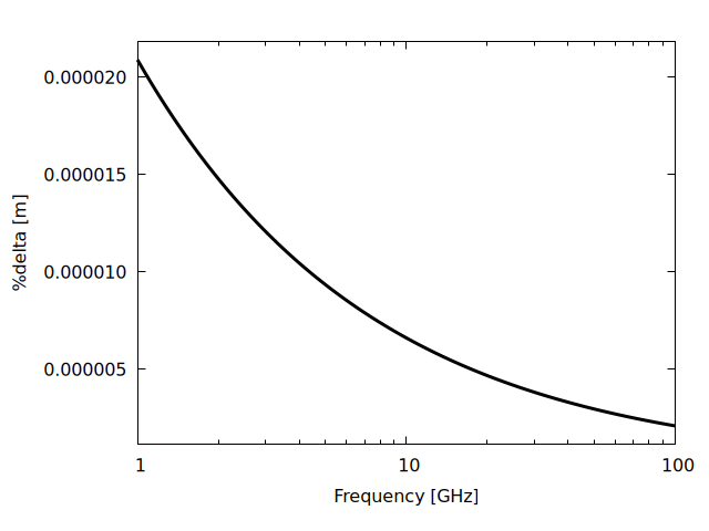

wxplot2d(8.686*%alpha(%mu_0,%sigma_Ti6Al4V,f*1e9),
    [f,75,110],
    [legend,false],
    [xlabel,"Frequency [GHz]"],
    [ylabel,"%alpha [dB/m]"],
    [style,[lines,3,11]],
    [gnuplot_preamble,"set grid"])$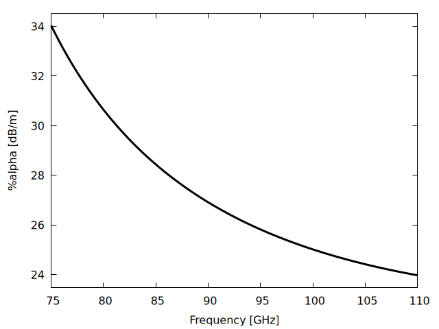

wxplot2d(%beta(f*1e9),
    [f,75,110],
    [legend,false],
    [xlabel,"Frequency [GHz]"],
    [ylabel,"%beta [rad/m]"],
    [style,[lines,3,11]],
    [gnuplot_preamble,"set grid"])$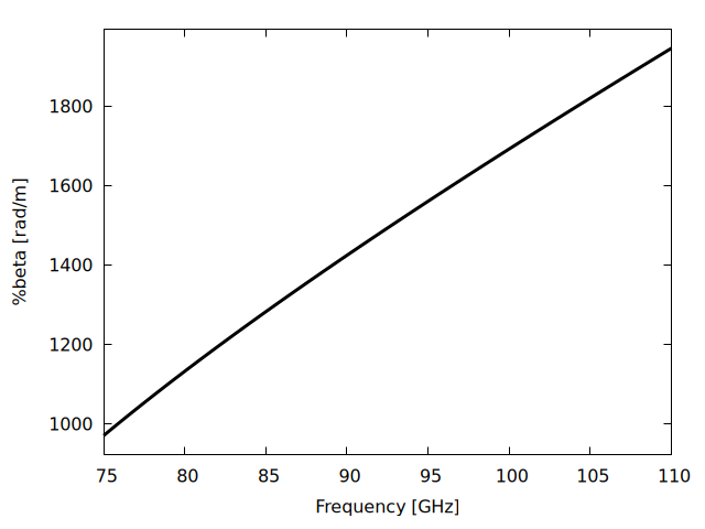

wxplot2d(Z_TE10(f*1e9),
    [f,75,110],
    [legend,false],
    [xlabel,"Frequency [GHz]"],
    [ylabel,"Z_TE10 [Ohm]"],
    [style,[lines,3,11]],
    [gnuplot_preamble,"set grid"])$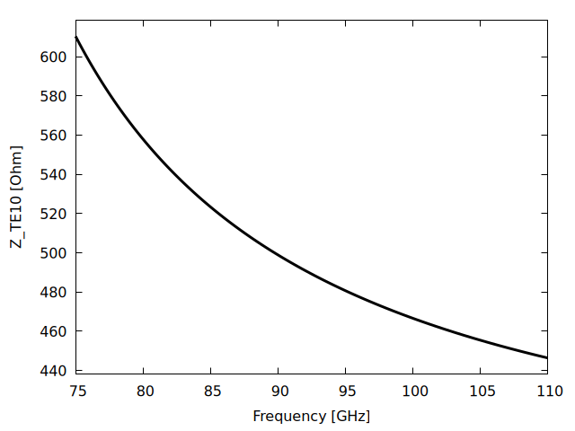

Figures of Merit with Surface Roughness

References:
- Ansoft HFSS 11, HFSS Online Help - Technical Notes, p 16-84

K_w(%delta,R_q):=1+exp(-(%delta/(2*R_q))^1.6);
%sigma_c(%sigma,K_w):=%sigma/K_w^2;

\mathit{K}_{w}\left(\delta , \mathit{R}_{q}\right):=1+\exp \left(-\left({{\delta}\over{2\,\mathit{R}_{q}}}\right)^{1.6}\right)

\sigma_{c}\left(\sigma , \mathit{K}_{w}\right):={{\sigma}\over{\mathit{K}_{w}^2}}

f_c;
float(Z_TE10(f_0));
float(%delta(%mu_0,%sigma_Ti6Al4V,2*%pi*f_0));
float(R_s(%delta(%mu_0,%sigma_Ti6Al4V,2*%pi*f_0),%sigma_Ti6Al4V));
float(8.686*%alpha(%mu_0,%sigma_Ti6Al4V,f_0));
float(K_w(%delta(%mu_0,%sigma_Ti6Al4V,2*%pi*f_0),R_q));
float(%sigma_Ti6Al4V_rough:%sigma_c(%sigma_Ti6Al4V,K_w(%delta(%mu_0,%sigma_Ti6Al4V,2*%pi*f_0),R_q)))$
float(R_s(%delta(%mu_0,%sigma_Ti6Al4V,2*%pi*f_0),%sigma_Ti6Al4V_rough));
float(8.686*%alpha(%mu_0,%sigma_Ti6Al4V_rough,f_0));

5.901488930968823 \times 10^{+10}

484.0102449848252

2.155471118561755 \times 10^{-6}

0.7998891361554963

26.01005660394874

1.454392527845496

1.691971594449821

37.82883197362146

wxplot2d([%sigma_Ti6Al4V,%sigma_c(%sigma_Ti6Al4V,K_w(%delta(%mu_0,%sigma_Ti6Al4V,2*%pi*f),R_q))],
    [f,1e6,1e11],
    [logx],
    [legend,false],
    [xlabel,"Frequency [Hz]"],
    [ylabel,"%sigma [S/m]"],
    [style,[lines,3,1],[lines,3,2]],
    [gnuplot_preamble,"set grid"])$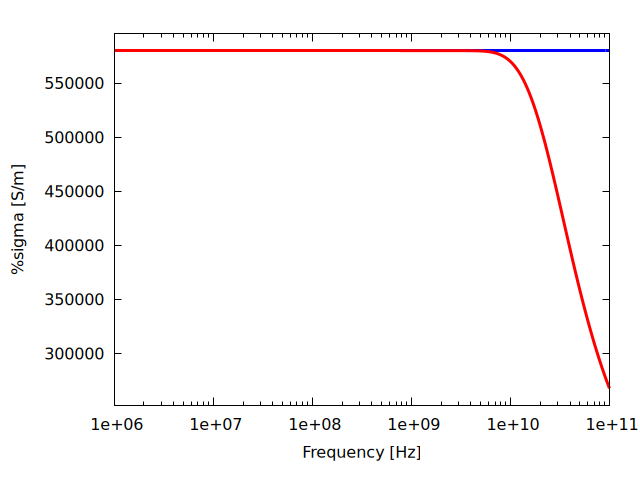

wxplot2d([8.686*%alpha(%mu_0,%sigma_Ti6Al4V,f*1e9),8.686*%alpha(%mu_0,%sigma_c(%sigma_Ti6Al4V,K_w(%delta(%mu_0,%sigma_Ti6Al4V,2*%pi*f*1e9),R_q)),f*1e9)],
    [f,75,110],
    [legend,false],
    [xlabel,"Frequency [GHz]"],
    [ylabel,"%alpha [dB/m]"],
    [style,[lines,3,11]],
    [gnuplot_preamble,"set grid"])$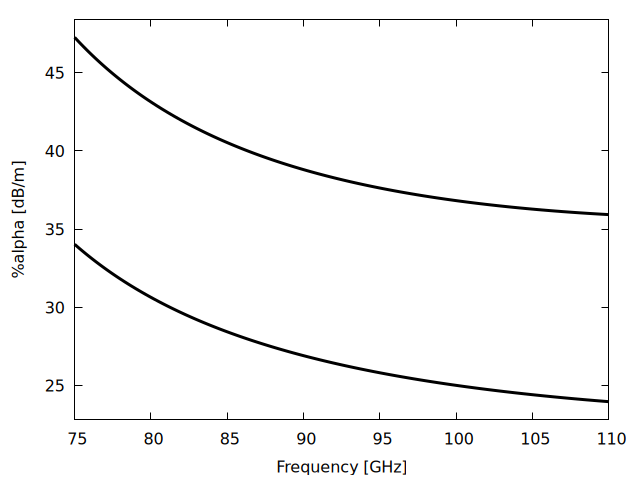

S-Parameters

l:0.05$

/* Reference impedance for the S-parameters.  0.2.4 set Z_0 := Z_TE10(f),
   i.e. it referred the line to its own characteristic impedance at every
   frequency.  That forces S11 = 0 identically, so the S11 Smith chart was a
   single point at the origin.  Refer instead to the TE10 wave impedance at
   band centre, which is what a fixed-impedance measurement sees.
   Note the LOCAL Z_0 in the block: 0.2.4 clobbered the global Z_0. */
Z_REF:float(Z_TE10(f_0));

define(S_WG(f),
    block([Z_0],
        Z_0:Z_REF,
        ABCD2S(
            ABCD_LossyTL(
                %alpha(%mu_0,%sigma_c(%sigma_Ti6Al4V,K_w(%delta(%mu_0,%sigma_Ti6Al4V,2*%pi*f),R_q)),f)+%i*%beta(f),
                l,
                Z_TE10(f)))))$

484.0102449848252

realpart(S_WG(f)) and imagpart(S_WG(f)) are symbolic expressions of roughly 300 000 characters, and plot2d re-does symbolic work at every sample point, so plotting them parametrically never finishes. Evaluate the S-parameter NUMERICALLY at each frequency first and plot the resulting point list: one evaluation is about 50 ms, so a hundred points take a few seconds.

S_WG_points(i,j,f1,f2,n):=makelist(
    block([z:ev(S_WG(fr)[i,j], numer)], [realpart(z), imagpart(z)]),
    fr, makelist(f1+(f2-f1)*kk/n, kk, 0, n))$
S11_pts:S_WG_points(1,1,75e9,110e9,100)$
S21_pts:S_WG_points(2,1,75e9,110e9,100)$

PlotSmithChart([discrete, S11_pts]);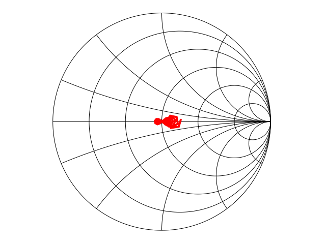

/* S21 is a TRANSMISSION coefficient; a Smith chart maps REFLECTION
   coefficient, so plot insertion loss against frequency instead -- again
   from the numerically evaluated points, for the reason given above. */
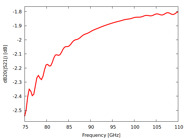
S21_dB:makelist([75+(110-75)*kk/100,
                 20*log10(sqrt(S21_pts[kk+1][1]^2+S21_pts[kk+1][2]^2))],
                kk, 0, 100)$
wxplot2d([discrete, S21_dB],
    [legend,false],
    [xlabel,"Frequency [GHz]"],
    [ylabel,"dB20(|S21|) [dB]"],
    [style,[lines,3,2]],
    [gnuplot_preamble,"set grid"]);