Appendix 1: AT-Cut alpha-Quartz Resonator

(See: Microsystem Design by Stephen D. Senturia, pp. 192-193, 570-577)
(See: An Introduction to the Theory of Piezoelectricity by Jiashi Yang, pp. 89-93)

1 Linear Piezoelectricity

1.1 Displacement (u), Strain (S), and Stress (T)

u: displacement [m]

(%i1) u:matrix([u_x(x,y,z,t)],[u_y(x,y,z,t)],[u_z(x,y,z,t)])$
u2S(u):=matrix([diff(u[1,1],x)],[diff(u[2,1],y)],[diff(u[3,1],z)],[diff(u[2,1],z)+diff(u[3,1],y)],[diff(u[1,1],z)+diff(u[3,1],x)],[diff(u[1,1],y)+diff(u[2,1],x)])$

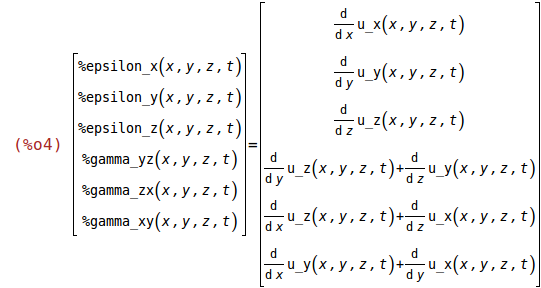
S: strain [] (%epsilon: normal strain, %gamma: shear strain)

(%i3) S:matrix([%epsilon_x(x,y,z,t)],[%epsilon_y(x,y,z,t)],[%epsilon_z(x,y,z,t)],[%gamma_yz(x,y,z,t)],[%gamma_zx(x,y,z,t)],[%gamma_xy(x,y,z,t)])$
S=u2S(u);

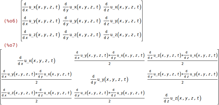
(%i5) grad(u):=matrix([diff(u[1,1],x,1),diff(u[1,1],y,1),diff(u[1,1],z,1)],[diff(u[2,1],x,1),diff(u[2,1],y,1),diff(u[2,1],z,1)],[diff(u[3,1],x,1),diff(u[3,1],y,1),diff(u[3,1],z,1)])$
grad(u);
1/2*(grad(u)+transpose(grad(u)));

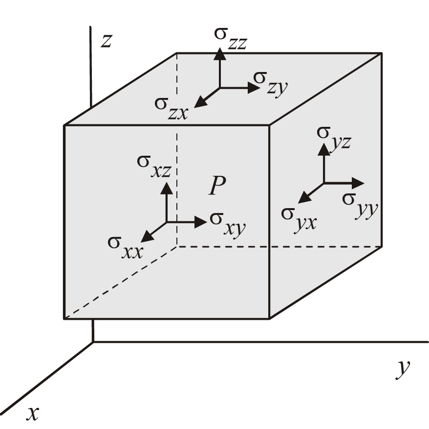
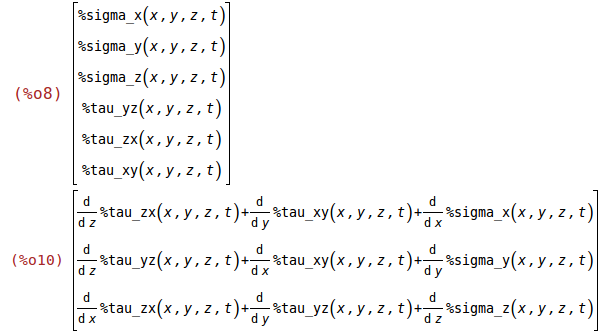
T: stress, force per unit area [N/m^2] (%sigma: normall stress, %tau: shear stress)

(%i8) T:matrix([%sigma_x(x,y,z,t)],[%sigma_y(x,y,z,t)],[%sigma_z(x,y,z,t)],[%tau_yz(x,y,z,t)],[%tau_zx(x,y,z,t)],[%tau_xy(x,y,z,t)]);
divT(T):=matrix([diff(T[1,1],x,1)+diff(T[6,1],y,1)+diff(T[5,1],z,1)],[diff(T[6,1],x,1)+diff(T[2,1],y,1)+diff(T[4,1],z,1)],[diff(T[5,1],x,1)+diff(T[4,1],y,1)+diff(T[3,1],z,1)])$
divT(T);

1.2 Electric Displacement (D) and Electric Field (E)

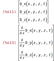
D: electric displacement [C/m^2]

(%i11) D:matrix([D_x(x,y,z,t)],[D_y(x,y,z,t)],[D_z(x,y,z,t)]);
divD(D):=matrix([diff(D[1,1],x,1)],[diff(D[2,1],y,1)],[diff(D[3,1],z,1)])$
divD(D);

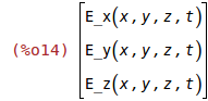
E: electric field [V/m]

(%i14) E:matrix([E_x(x,y,z,t)],[E_y(x,y,z,t)],[E_z(x,y,z,t)]);

1.3 Linear Constitutive Tensors

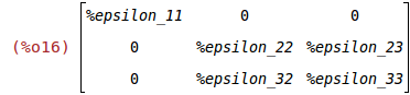
The number of independent non-zero constants depends on the crystal symmetry. Y-cut (AT-, BT-, ST-cut) alpha-quartz is a material of crystal class 32.

%epsilon: dielectric permittivity tensor [C/(V.m)] (at constant strain)

(%i15) declare([%epsilon_0,%epsilon_11,%epsilon_22,%epsilon_23,%epsilon_32,%epsilon_33],[constant,real,scalar])$
%epsilon:matrix([%epsilon_11,0,0],[0,%epsilon_22,%epsilon_23],[0,%epsilon_32,%epsilon_33]);

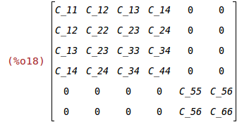
C: elastic stiffness tensor [N/m^2] (at constant electric field)

(%i17) declare([C_11,C_12,C_13,C_14,C_22,C_23,C_24,C_33,C_34,C_44,C_55,C_56,C_66],[constant,real,scalar])$
C:matrix([C_11, C_12, C_13, C_14, 0, 0],[C_12, C_22, C_23, C_24, 0, 0],[C_13, C_23, C_33, C_34, 0, 0],[C_14, C_24, C_34, C_44, 0, 0],[0, 0, 0, 0, C_55, C_56],[0, 0, 0, 0, C_56, C_66]);

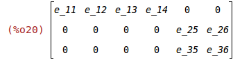
e: piezoelectricity tensor [C/m^2]

(%i19) declare([e_11,e_12,e_13,e_14,e_25,e_26,e_35,e_36],[constant,real,scalar])$
e:matrix([e_11,e_12,e_13,e_14,0,0],[0,0,0,0,e_25,e_26],[0,0,0,0,e_35,e_36]);

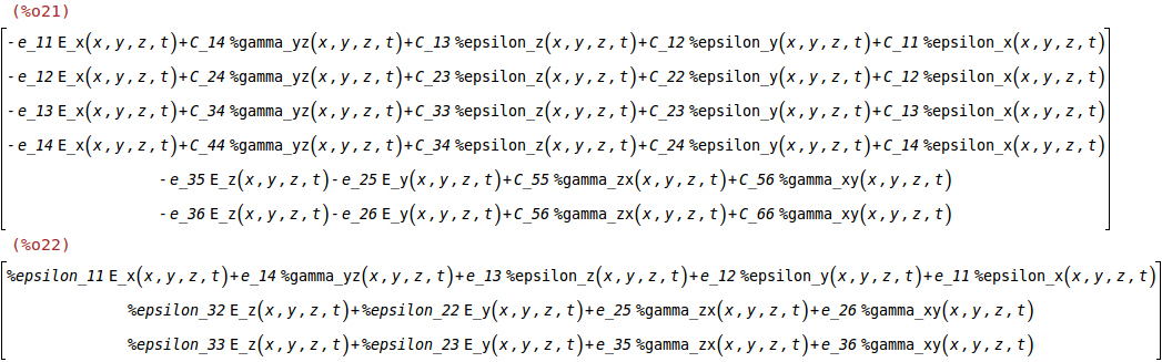
1.4 Lippmann's Linear Constitutive Equations in Charge-Stress Form

(%i21) T:C.S-transpose(e).E;
D:e.S+transpose(%epsilon).E;

Some of the most important resonator phenomena (e.g. acceleration sensitivity) are due to nonlinear effects. Quartz has numerous higher order constants, e.g., 14 third-order and 23 fourth-order elastic constants, as well as 16 third-order piezoelectric coefficients are known (Source: "Quartz Crystal Resonators and Oscillators for Frequency Control and Timing Applications - A Tutorial", by John R. Vig, November 2008.)

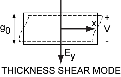
2 Boundary Value Problem

Assume a thickness-shear vibration of a AT-cut quartz plate around the Z-axis, excited by an electric field along the Y-axis.
Assume the plate can not move along the Y- and Z-axis: u_y(y,t)=0, u_z(y,t)=0.

(%i23) %epsilon_x(x,y,z,t):=0$
%epsilon_y(x,y,z,t):=0$
%epsilon_z(x,y,z,t):=0$
%gamma_yz(x,y,z,t):=0$
%gamma_xz(x,y,z,t):=0$
%gamma_xy(x,y,z,t):=diff(u_x(y,t),y,1)$

Assume the X- and Z-component of the electric field to be zero: E_x(x,y,z,t)=0, E_z(x,y,z,t)=0.

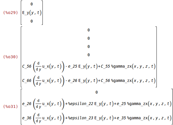
(%i29) E:matrix([0],[E_y(y,t)],[0]);
T:ev(C.S-transpose(e).E);
D:ev(e.S+transpose(%epsilon).E);

2.1 Potential Energy

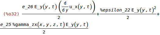
Electrostatic Energy Density, w_e

(%i32) w_e:expand(ev(1/2*transpose(E).D));

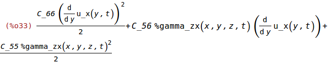
Elastic Energy Density, w_m

(%i33) w_m:expand(ev(1/2*transpose(S).C.S));

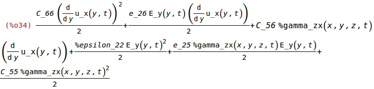
Total Energy Density

(%i34) w_t:w_e+w_m;

2.2 Newton's Law of Motion for a Continuum [PDE in Quartz Volume]

Force density

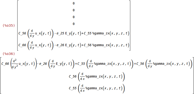
(%i35) ev(T);
f:ratsimp(divT(ev(T)));

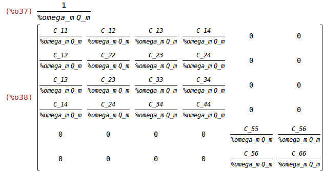
Viscosity and Q Factor

%eta: viscosity tensor [N/(m^2.s)]
%tau_m is the motional time constant
%omega_m is the mechanical resonant radian frequency
Q_m is the mechanical Q factor

(%i37) %tau_m:1/(%omega_m*Q_m);
%eta:%tau_m*C;

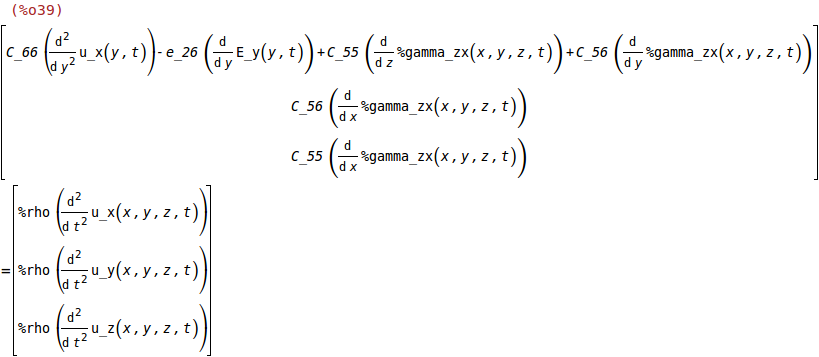
Newton's Equation of Motion

%rho: mass density [kg/m^3]

(%i39) f=%rho*diff(u,t,2);

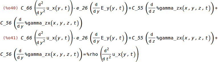
(%i40) f_x:ev(f[1,1]);
f_x=%rho*diff(u_x(y,t),t,2);

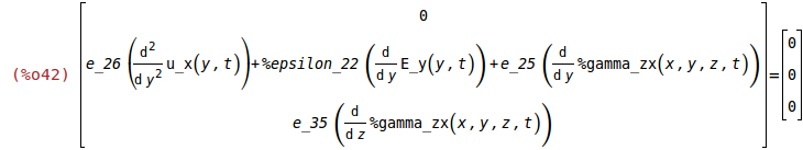
3 Gauss' Law [PDE in Quartz Volume]

(%i42) divD(ev(D))=matrix([0],[0],[0]);

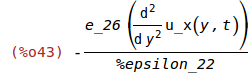
Calculating 'diff(E_y(y,t),y,1)

(%i43) -(e_26*('diff(u_x(y,t),y,2)))/%epsilon_22;

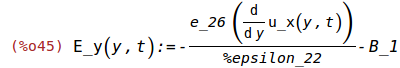
Calculating E_y(y,t)
B_1 is an integration constant.

(%i44) declare([B_1],[constant,real,scalar])$
define(E_y(y,t),-(e_26*(diff(u_x(y,t),y,1)))/%epsilon_22-B_1);

4 Boundary Conditions

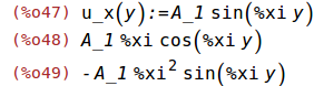
Assume a solution u_x(y,t):=A_1*sin(%xi*y)*exp(%i*%omega_m*t) with %xi:sqrt(%rho/(C_66*(1+k_26^2)))*%omega
k_26: sqrt(e_26^2/(%epsilon_22*C_66))

(%i46) declare([A_1],[constant,real,scalar])$
u_x(y):=A_1*sin(%xi*y);
ratsimp(diff(u_x(y),y,1));
ratsimp(diff(u_x(y),y,2));

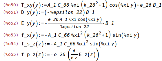
(%i50) define(T_xy(y),C_66*(1+k_26^2)*%th(2)+e_26*B_1);
D_y(y):=-%epsilon_22*B_1;
define(E_y(y),-(e_26*%th(4))/%epsilon_22-B_1);
define(f_x(y),C_66*(1+k_26^2)*%th(4));
define(f_s_z(z),C_66*%th(5));
define(f_p_z(z),-e_26*(diff(E_z(z),z,1)));

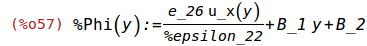
Calculating the potential %Phi(y)
B_2 is an integration constant.

(%i56) declare([B_2],[constant,real,scalar])$
%Phi(y):=e_26*u_x(y)/%epsilon_22+B_1*y+B_2;

%tau_xy(z=-g_0/2)=0,
%tau_xy(z=g_0/2)=0,
%Phi(z=g_0/2)-%Phi(z=-g_0/2)=V,
with,
g_0: thickness [m]
V: applied voltage [V]

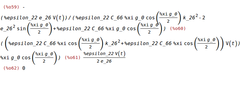
(%i58) solve([ev(T_xy(g_0/2))=0,ev(%Phi(g_0/2)-%Phi(-g_0/2))=V(t)],[A_1,B_1])$
A_1:ratsimp(ev(A_1,%));
B_1:ratsimp(ev(B_1,%th(2)));
ratsimp(ev(A_1,%xi=%pi/g_0));
ratsimp(ev(B_1,%xi=%pi/g_0));

5 Elastic Wave Equation and Christoffel Equation

(See: http://sepwww.stanford.edu/public/docs/sep92/hector1/paper_html/node2.html)

(%i63) K:ev(1/k*matrix([k_x,0,0,0,k_z,k_y],[0,k_y,0,k_z,0,k_x],[0,0,k_z,k_y,k_x,0]),k_x=0,k_z=0);
k:ev(sqrt(k_x^2+k_y^2+k_z^2),k_x=0,k_z=0);

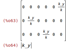
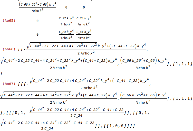
(%i65) M:ratsimp(k^2/%rho*K.subst(C_66*(1+k_26^2),C_66,C).transpose(K));
ratsimp(eigenvalues(M));
ratsimp(eigenvectors(M));

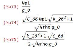
The vibration frequency of the thickness-shear mode, f_m, can be used to determine the thickness of the Y-cut alpha-quartz plate, g_0

(%i68) declare([%rho,C_66,g_0,k_26],[constant,real,scalar])$
assume(%rho>0)$
assume(C_66>0)$
assume(g_0>0)$
assume(k_26>0)$
k_y:2*%pi/(2*g_0);
%omega_m:sqrt(ev((k_y^2*C_66*(1+k_26^2))/(%rho)));
f_m:1/(2*%pi)*%omega_m;

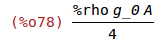
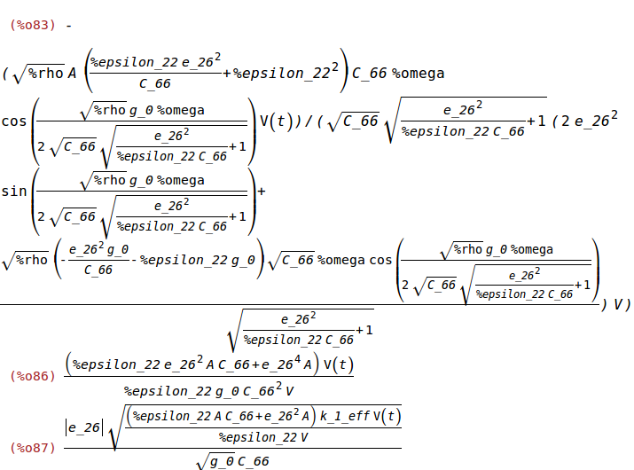
m is the effective mass.
A is the electrode area.

(%i76) declare([A],[constant,real,scalar])$
m:A*integrate(u_x(y)^2*%rho,y,0,g_0/2)/A_1^2$
m:ev(m,%xi=sqrt(%rho/(C_66*(1+k_26^2)))*%omega_m);

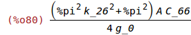
k_1_eff is the linear spring constant.

(%i79) solve([%omega_m=sqrt(k_1_eff/m)],[k_1_eff])$
ev(k_1_eff,%);

Tf is the linear temperature coefficient of frequency.

(%i81) Tf:'diff(log(f_m),Temp);

6 Charge, q, on the Electrodes

Boundary condition for D
A is the electrode area.

(%i82) q:ratsimp(-D_y(g_0/2)*A);

7 Motional Capacitance, C_m, Static Capacitance, C_0, and Transduction Factor, %eta

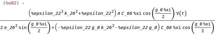
(%i83) C_XTAL:ev(q/V,
    %xi=sqrt(%rho/(C_66*(1+e_26^2/(%epsilon_22*C_66))))*%omega,
    k_26=sqrt(e_26^2/(%epsilon_22*C_66)));
C_0:ratsimp(limit(C_XTAL,%omega,0));
ratsimp(C_XTAL-C_0)$
C_m:ratsimp(ev(k_26^2*C_0,
    k_26=sqrt(e_26^2/(%epsilon_22*C_66))));
%eta:ratsimp(ev(sqrt(k_26^2*k_1_eff*C_0),
    k_26=sqrt(e_26^2/(%epsilon_22*C_66))));

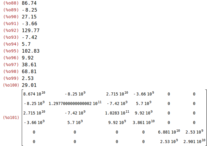
8 Material Parameters

8.1 AT-Cut alpha-Quartz (Trigonal Structure, Crystal Class 32)

(See "Elastic and Piezoelectric Constants of Alpha-Quartz", by R. Bechmann, American Physical Society Phys. Rev., vol. 110, no. 5, pp. 1060-1061, June 1958)

(%i88) C_11:86.74;
C_12:-8.25;
C_13:27.15;
C_14:-3.66;
C_22:129.77;
C_23:-7.42;
C_24:5.70;
C_33:102.83;
C_34:9.92;
C_44:38.61;
C_55:68.81;
C_56:2.53;
C_66:29.01;
C:1e9*matrix([C_11, C_12, C_13, C_14, 0, 0],[C_12, C_22, C_23, C_24, 0, 0],[C_13, C_23, C_33, C_34, 0, 0],[C_14, C_24, C_34, C_44, 0, 0],[0, 0, 0, 0, C_55, C_56],[0, 0, 0, 0, C_56, C_66]);

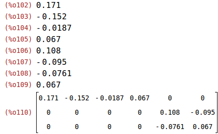
(%i102) e_11:0.171;
e_12:-0.152;
e_13:-0.0187;
e_14:0.067;
e_25:0.108;
e_26:-0.095;
e_35:-0.0761;
e_36:0.067;
e:matrix([e_11,e_12,e_13,e_14,0,0],[0,0,0,0,e_25,e_26],[0,0,0,0,e_35,e_36]);

(%i111) %epsilon_11:39.21;
%epsilon_22:39.82;
%epsilon_23:0.86;
%epsilon_32:0.86;
%epsilon_33:40.42;
%epsilon:1e-12*matrix([%epsilon_11,0,0],[0,%epsilon_22,%epsilon_23],[0,%epsilon_32,%epsilon_33]);

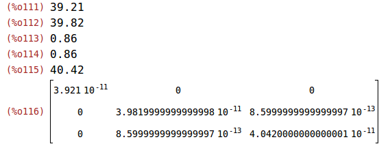
(%i117) %rho:2650.67;

k: piezoelectric coupling coefficient

(%i118) k_26:sqrt(e_26^2/(C_66*1e9*%epsilon_22*1e-12));
k_26^2;