/* Put rfMaxima.mac in the same directory as this notebook, or add its
   directory to file_search_maxima. */
load("rfMaxima.mac")$Real Transformer
Generated from LOSSY_TRANSFORMER.wxm with rfMaxima 0.2.5 on Maxima 5.46.0.
All results were computed by executing the notebook; none is transcribed.
4-Port Model of Real Transformer
4-Port Y-parameters of the real transformer
declare(k,real)$
declare(L1,real)$
declare(L2,real)$
declare(Z_0,real)$
assume(k>0)$
assume(L1>0)$
assume(L2>0)$
assume(Z_0>0)$
k is the coupling factor of the transformer. M is the mutual inductance of the transformer.
/* Mutual inductance of two coupled coils: M = k*sqrt(L1*L2).
   0.2.4 had sqrt(L1+L2) here.  (The 4-port Y-matrix below always used
   sqrt(L1*L2) correctly, so only this displayed definition was wrong.) */
M:k*sqrt(L1*L2);Y_REAL_TRANSFORMER:1/(1-k^2)*matrix(
[1/(s*L1),-1/(s*L1),-k/(s*sqrt(L1*L2)),k/(s*sqrt(L1*L2))],
[-1/(s*L1),1/(s*L1),k/(s*sqrt(L1*L2)),-k/(s*sqrt(L1*L2))],
[-k/(s*sqrt(L1*L2)),k/(s*sqrt(L1*L2)),1/(s*L2),-1/(s*L2)],
[k/(s*sqrt(L1*L2)),-k/(s*sqrt(L1*L2)),-1/(s*L2),1/(s*L2)]);Y_REAL_TRANSFORMER.matrix([v1],[v2],[v3],[v4]);2-Port parameters of the real transformer
Solution:linsolve([
i1=(k*v4)/((1-k^2)*s*sqrt(L1*L2))-(k*v3)/((1-k^2)*s*sqrt(L1*L2))-v2/((1-k^2)*s*L1)+v1/((1-k^2)*s*L1),
i2=-(k*v4)/((1-k^2)*s*sqrt(L1*L2))+(k*v3)/((1-k^2)*s*sqrt(L1*L2))+v2/((1-k^2)*s*L1)-v1/((1-k^2)*s*L1),
i3=(k*v2)/((1-k^2)*s*sqrt(L1*L2))-(k*v1)/((1-k^2)*s*sqrt(L1*L2))-v4/((1-k^2)*s*L2)+v3/((1-k^2)*s*L2),
i4=-(k*v2)/((1-k^2)*s*sqrt(L1*L2))+(k*v1)/((1-k^2)*s*sqrt(L1*L2))+v4/((1-k^2)*s*L2)-v3/((1-k^2)*s*L2),
v2=0,
v4=0,
i2=-i1,
i4=-i3,
v1=v_in,
v3=v_out,
i1=i_in,
i3=i_out],[i1,i2,i3,i4,v1,v2,v3,v4,i_in,i_out]);TwoPortMatrices(Solution);ABCD(s) :=
G(s) :=
H(s) :=
InverseABCD(s) :=
S(s) :=
Y(s) :=
Z(s) :=
SParameters(S);Abs_S11(%omega) :=
Arg_S11(%omega) :=
Abs_S12(%omega) :=
Arg_S12(%omega) :=
Abs_S21(%omega) :=
Arg_S21(%omega) :=
tau_g(%omega) :=
Abs_S22(%omega) :=
Arg_S22(%omega) :=
Z_IN(s) :=
R_IN(%omega) :=
X_IN(%omega) :=
Z_OUT(s) :=
R_OUT(%omega) :=
X_OUT(%omega) :=
2-Port Model of Capacitively-Tuned Real Transformer
declare(C,real)$
assume(C>0)$
Solution:linsolve([
i1=(k*v4)/((1-k^2)*s*sqrt(L1*L2))-(k*v3)/((1-k^2)*s*sqrt(L1*L2))-v2/((1-k^2)*s*L1)+v1/((1-k^2)*s*L1),
i2=-(k*v4)/((1-k^2)*s*sqrt(L1*L2))+(k*v3)/((1-k^2)*s*sqrt(L1*L2))+v2/((1-k^2)*s*L1)-v1/((1-k^2)*s*L1),
i3=(k*v2)/((1-k^2)*s*sqrt(L1*L2))-(k*v1)/((1-k^2)*s*sqrt(L1*L2))-v4/((1-k^2)*s*L2)+v3/((1-k^2)*s*L2),
i4=-(k*v2)/((1-k^2)*s*sqrt(L1*L2))+(k*v1)/((1-k^2)*s*sqrt(L1*L2))+v4/((1-k^2)*s*L2)-v3/((1-k^2)*s*L2),
v2=0,
v4=0,
i2=-i1,
i4=-i3,
v_in=v1,
v_out=v3,
v_in=1/(s*C)*i5,
i_in=i5+i1,
i_out=i3],[i1,i2,i3,i4,i5,v1,v2,v3,v4,i_in,i_out]);TwoPortMatrices(Solution);ABCD(s) :=
G(s) :=
H(s) :=
InverseABCD(s) :=
S(s) :=
Y(s) :=
Z(s) :=
SParameters(S);Abs_S11(%omega) :=
Arg_S11(%omega) :=
Abs_S12(%omega) :=
Arg_S12(%omega) :=
Abs_S21(%omega) :=
Arg_S21(%omega) :=
tau_g(%omega) :=
Abs_S22(%omega) :=
Arg_S22(%omega) :=
Z_IN(s) :=
R_IN(%omega) :=
X_IN(%omega) :=
Z_OUT(s) :=
R_OUT(%omega) :=
X_OUT(%omega) :=
2-Port Model of Capacitively-Tuned Real and Lossy Transformer
declare(R1,real)$
declare(R2,real)$
assume(R1>0)$
assume(R2>0)$
Solution:linsolve([
i1=(k*v4)/((1-k^2)*s*sqrt(L1*L2))-(k*v3)/((1-k^2)*s*sqrt(L1*L2))-v2/((1-k^2)*s*L1)+v1/((1-k^2)*s*L1),
i2=-(k*v4)/((1-k^2)*s*sqrt(L1*L2))+(k*v3)/((1-k^2)*s*sqrt(L1*L2))+v2/((1-k^2)*s*L1)-v1/((1-k^2)*s*L1),
i3=(k*v2)/((1-k^2)*s*sqrt(L1*L2))-(k*v1)/((1-k^2)*s*sqrt(L1*L2))-v4/((1-k^2)*s*L2)+v3/((1-k^2)*s*L2),
i4=-(k*v2)/((1-k^2)*s*sqrt(L1*L2))+(k*v1)/((1-k^2)*s*sqrt(L1*L2))+v4/((1-k^2)*s*L2)-v3/((1-k^2)*s*L2),
v2=0,
v4=0,
i2=-i1,
i4=-i3,
v0-v1=R1*i_in,
v_in=v0,
v_out=v5,
v5-v3=R2*i_out,
v_in=1/(s*C)*i5,
i_in=i5+i1,
i_out=i3],[i1,i2,i3,i4,i5,v0,v1,v2,v3,v4,v5,i_in,i_out]);TwoPortMatrices(Solution);ABCD(s) :=
G(s) :=
H(s) :=
InverseABCD(s) :=
S(s) :=
Y(s) :=
Z(s) :=
SParameters(S);Abs_S11(%omega) :=
Arg_S11(%omega) :=
Abs_S12(%omega) :=
Arg_S12(%omega) :=
Abs_S21(%omega) :=
Arg_S21(%omega) :=
tau_g(%omega) :=
Abs_S22(%omega) :=
Arg_S22(%omega) :=
Z_IN(s) :=
R_IN(%omega) :=
X_IN(%omega) :=
Z_OUT(s) :=
R_OUT(%omega) :=
X_OUT(%omega) :=
L1:2e-9$
L2:2e-9$
k:0.9$
Z_0:50$
fres:2e9$
C:1/((2*%pi*fres)^2*L1)$
float(C);
Q1:10$
Q2:10$
R1:2*%pi*fres*L1/Q1$
float(R1);
R2:2*%pi*fres*L2/Q2$
float(R2);PlotSmithChart([
parametric,
realpart(S(%i*2*%pi*f)[1,1]),
imagpart(S(%i*2*%pi*f)[1,1]),
[f,1e6,20e9],
[nticks,100]]);
/* S12 is a TRANSMISSION coefficient; a Smith chart maps REFLECTION
coefficient. Its magnitude is plotted against frequency further down. */
/* S21 is a TRANSMISSION coefficient; a Smith chart maps REFLECTION
coefficient. Its magnitude is plotted against frequency further down. */
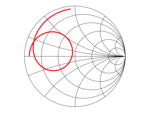
PlotSmithChart([
parametric,
realpart(S(%i*2*%pi*f)[2,2]),
imagpart(S(%i*2*%pi*f)[2,2]),
[f,1e6,20e9],
[nticks,100]]);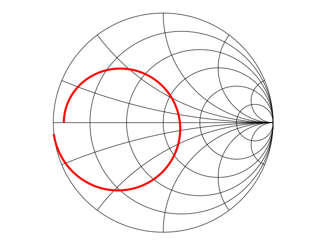
wxplot2d(ev(20*log10(Abs_S11(2*%pi*f*1e9))),
[f,0.1,20],
[legend,false],
[xlabel,"Frequency [GHz]"],
[ylabel,"dB20(|S11|)"],
[style,[lines,3,2]],
[gnuplot_preamble,"set grid"])$
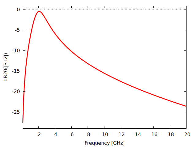
wxplot2d(ev(20*log10(Abs_S12(2*%pi*f*1e9))),
[f,0.1,20],
[legend,false],
[xlabel,"Frequency [GHz]"],
[ylabel,"dB20(|S12|)"],
[style,[lines,3,2]],
[gnuplot_preamble,"set grid"])$
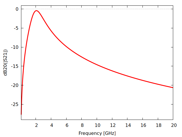
wxplot2d(ev(20*log10(Abs_S21(2*%pi*f*1e9))),
[f,0.1,20],
[legend,false],
[xlabel,"Frequency [GHz]"],
[ylabel,"dB20(|S21|)"],
[style,[lines,3,2]],
[gnuplot_preamble,"set grid"])$
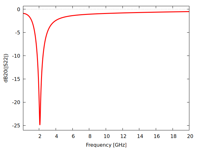
wxplot2d(ev(20*log10(Abs_S22(2*%pi*f*1e9))),
[f,0.1,20],
[legend,false],
[xlabel,"Frequency [GHz]"],
[ylabel,"dB20(|S22|)"],
[style,[lines,3,2]],
[gnuplot_preamble,"set grid"])$
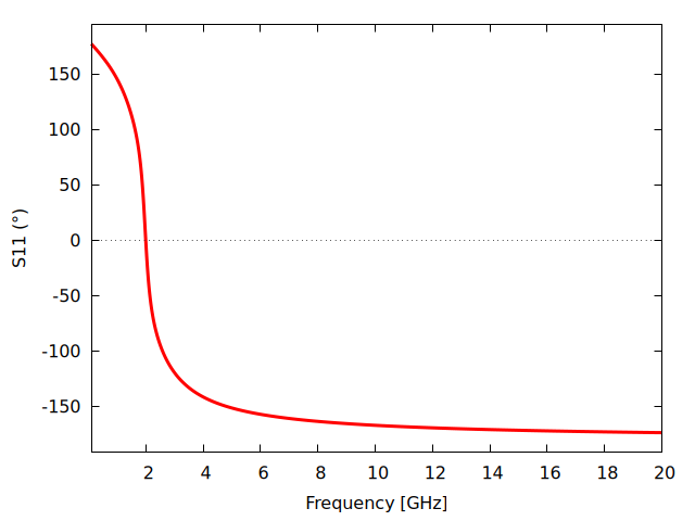
wxplot2d(ev(Arg_S11(2*%pi*f*1e9)*180/%pi),
[f,0.1,20],
[legend,false],
[xlabel,"Frequency [GHz]"],
[ylabel,"S11 (°)"],
[style,[lines,3,2]],
[gnuplot_preamble,"set grid"])$
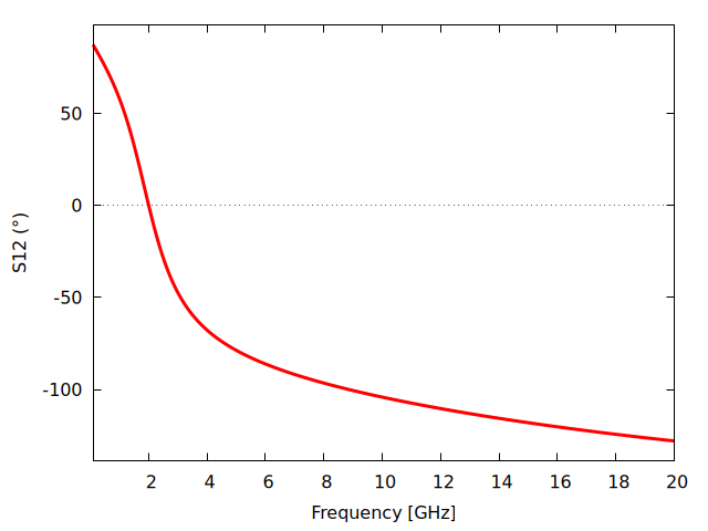
wxplot2d(ev(Arg_S12(2*%pi*f*1e9)*180/%pi),
[f,0.1,20],
[legend,false],
[xlabel,"Frequency [GHz]"],
[ylabel,"S12 (°)"],
[style,[lines,3,2]],
[gnuplot_preamble,"set grid"])$
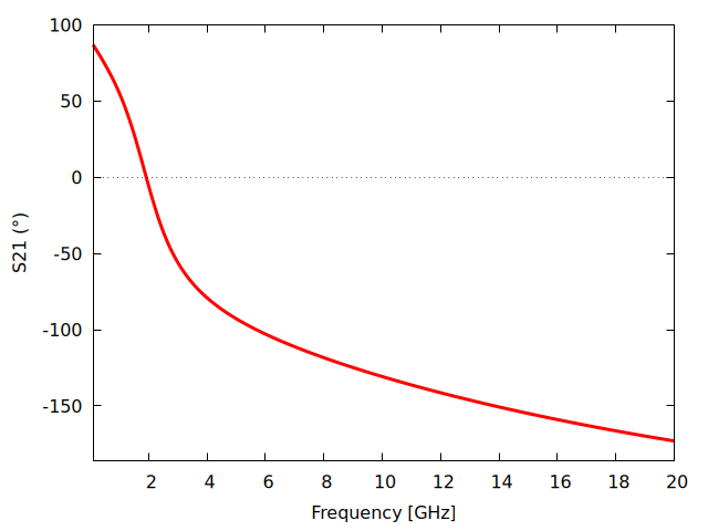
wxplot2d(ev(Arg_S21(2*%pi*f*1e9)*180/%pi),
[f,0.1,20],
[legend,false],
[xlabel,"Frequency [GHz]"],
[ylabel,"S21 (°)"],
[style,[lines,3,2]],
[gnuplot_preamble,"set grid"])$
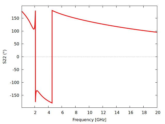
wxplot2d(ev(Arg_S22(2*%pi*f*1e9)*180/%pi),
[f,0.1,20],
[legend,false],
[xlabel,"Frequency [GHz]"],
[ylabel,"S22 (°)"],
[style,[lines,3,2]],
[gnuplot_preamble,"set grid"])$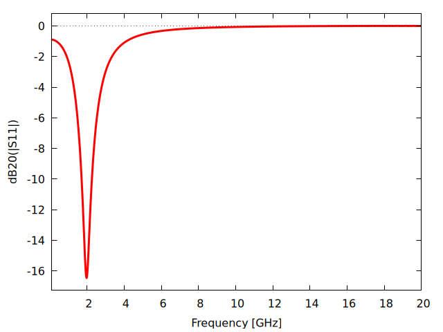
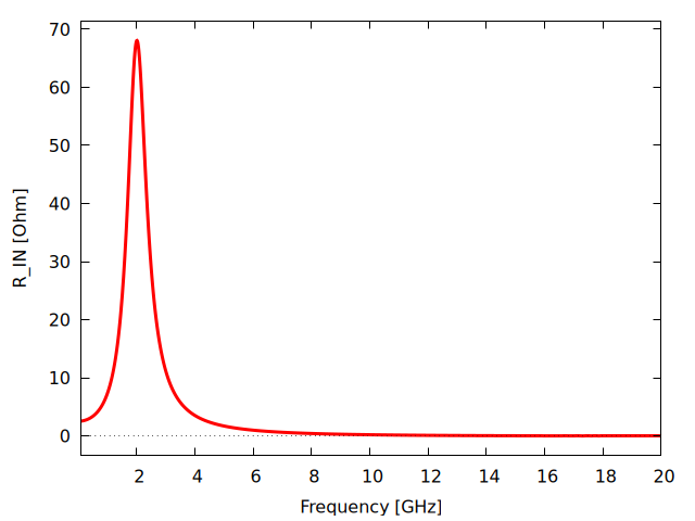
wxplot2d(ev((R_IN(2*%pi*f*1e9))),
[f,0.1,20],
[legend,false],
[xlabel,"Frequency [GHz]"],
[ylabel,"R_IN [Ohm]"],
[style,[lines,3,2]],
[gnuplot_preamble,"set grid"])$
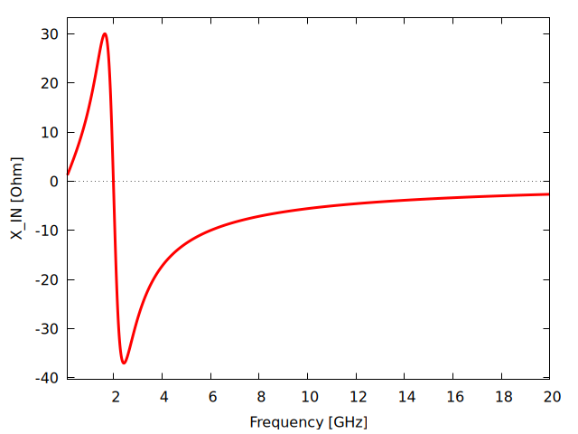
wxplot2d(ev((X_IN(2*%pi*f*1e9))),
[f,0.1,20],
[legend,false],
[xlabel,"Frequency [GHz]"],
[ylabel,"X_IN [Ohm]"],
[style,[lines,3,2]],
[gnuplot_preamble,"set grid"]);
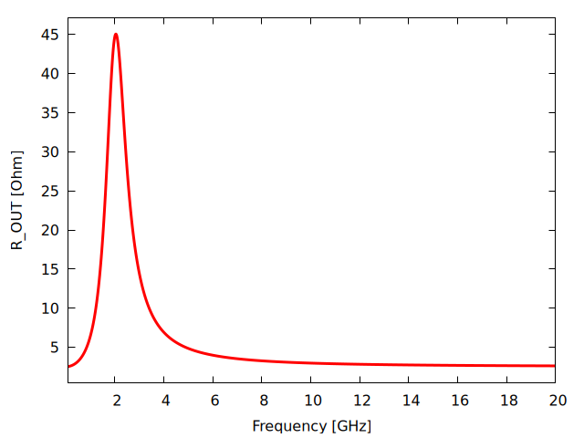
wxplot2d(ev((R_OUT(2*%pi*f*1e9))),
[f,0.1,20],
[legend,false],
[xlabel,"Frequency [GHz]"],
[ylabel,"R_OUT [Ohm]"],
[style,[lines,3,2]],
[gnuplot_preamble,"set grid"])$
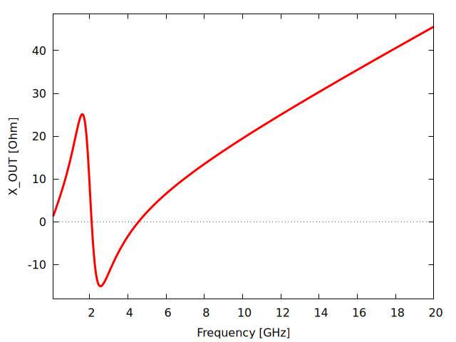
wxplot2d(ev((X_OUT(2*%pi*f*1e9))),
[f,0.1,20],
[legend,false],
[xlabel,"Frequency [GHz]"],
[ylabel,"X_OUT [Ohm]"],
[style,[lines,3,2]],
[gnuplot_preamble,"set grid"])$
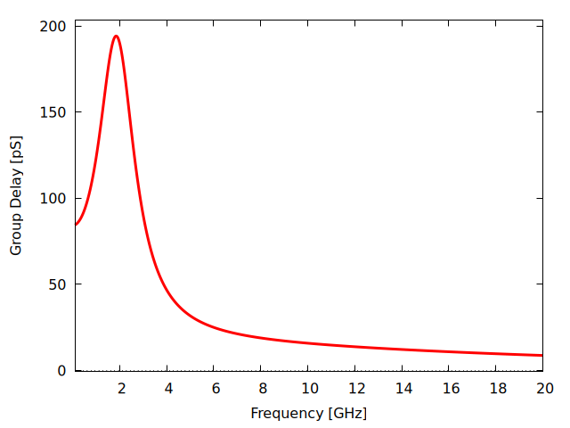
wxplot2d(ev((tau_g(2*%pi*f*1e9))*1e12),
[f,0.1,20],
[legend,false],
[xlabel,"Frequency [GHz]"],
[ylabel,"Group Delay [pS]"],
[style,[lines,3,2]],
[gnuplot_preamble,"set grid"])$