2nd Order Butterworth Filter, Implemented Using Sallen–Key Topology

Generated from BUTTERWORTH.wxm with rfMaxima 0.2.5 on Maxima 5.46.0. All results were computed by executing the notebook; none is transcribed.

/* Put rfMaxima.mac in the same directory as this notebook, or add its
   directory to file_search_maxima. */
load("rfMaxima.mac")$

(see https://en.wikipedia.org/wiki/Butterworth_filter)

Filter Design

declare([C_1,C_2,R_1,R_2,%omega_b,%omega_c],[constant,real,scalar])$
assume(C_1>0)$
assume(C_2>0)$
assume(R_1>0)$
assume(R_2>0)$
assume(%omega_b>0)$
assume(%omega_c>0)$

G(s):=1/(1+C_2*(R_1+R_2)*s+C_1*C_2*R_1*R_2*s^2);
/* abs() of a symbolic complex expression does not expand into
   realpart^2 + imagpart^2 by itself, so take the parts explicitly. */
block([D],D:ev(denom(G(s)),s=%i*%omega),expand(realpart(D)^2+imagpart(D)^2));

G\left(s\right):={{1}\over{1+C_{2}\,\left(R_{1}+R_{2}\right)\,s+C_{1}\,C_{2}\,R_{1}\,R_{2}\,s^2}}

C_{1}^2\,C_{2}^2\,R_{1}^2\,R_{2}^2\,\omega^4+C_{2}^2\,R_{2}^2\,\omega^2+2\,C_{2}^2\,R_{1}\,R_{2}\,\omega^2-2\,C_{1}\,C_{2}\,R_{1}\,R_{2}\,\omega^2+C_{2}^2\,R_{1}^2\,\omega^2+1

solve([%omega_c^4=1/(C_1^2*C_2^2*R_1^2*R_2^2),C_2^2*R_2^2+2*C_2^2*R_1*R_2-2*C_1*C_2*R_1*R_2+C_2^2*R_1^2=0],[C_1,C_2,R_1,R_2]);

\left[ \left[ C_{1}=-{{\sqrt{2}\,i\,\%r_{2}+\sqrt{2}\,i\,\%r_{1}}\over{2\,\omega_{c}\,\%r_{1}\,\%r_{2}}} , C_{2}=-{{\sqrt{2}\,i}\over{\omega_{c}\,\%r_{2}+\omega_{c}\,\%r_{1}}} , R_{1}=\%r_{1} , R_{2}=\%r_{2} \right] , \left[ C_{1}={{\sqrt{2}\,i\,\%r_{4}+\sqrt{2}\,i\,\%r_{3}}\over{2\,\omega_{c}\,\%r_{3}\,\%r_{4}}} , C_{2}={{\sqrt{2}\,i}\over{\omega_{c}\,\%r_{4}+\omega_{c}\,\%r_{3}}} , R_{1}=\%r_{3} , R_{2}=\%r_{4} \right] , \left[ C_{1}=-{{\sqrt{2}\,\%r_{6}+\sqrt{2}\,\%r_{5}}\over{2\,\omega_{c}\,\%r_{5}\,\%r_{6}}} , C_{2}=-{{\sqrt{2}}\over{\omega_{c}\,\%r_{6}+\omega_{c}\,\%r_{5}}} , R_{1}=\%r_{5} , R_{2}=\%r_{6} \right] , \left[ C_{1}={{\sqrt{2}\,\%r_{8}+\sqrt{2}\,\%r_{7}}\over{2\,\omega_{c}\,\%r_{7}\,\%r_{8}}} , C_{2}={{\sqrt{2}}\over{\omega_{c}\,\%r_{8}+\omega_{c}\,\%r_{7}}} , R_{1}=\%r_{7} , R_{2}=\%r_{8} \right] \right]

We have two degrees of freedom to realize the 2nd order Butterworth filter, given %omega_c. Let us therefore assume R_1=1000 Ohm and R_2=1000 Ohm.

Butterworth:ev([C_1=(%r8+%r7)/(sqrt(2)*%omega_c*%r7*%r8),C_2=sqrt(2)/(%omega_c*%r8+%omega_c*%r7),R_1=%r7,R_2=%r8],%r7=1000,%r8=1000);

\left[ C_{1}={{1}\over{125\,2^{{{5}\over{2}}}\,\omega_{c}}} , C_{2}={{1}\over{125\,2^{{{7}\over{2}}}\,\omega_{c}}} , R_{1}=1000 , R_{2}=1000 \right]

define(G_REALIZED(s),ratsimp(ev(G(s),C_1=ev(C_1,Butterworth),C_2=ev(C_2,Butterworth),R_1=ev(R_1,Butterworth),R_2=ev(R_2,Butterworth))));

\mathit{G}_{REALIZED}\left(s\right):={{\omega_{c}^2}\over{s^2+\sqrt{2}\,\omega_{c}\,s+\omega_{c}^2}}

ratsimp(ev(abs(G_REALIZED(s))^2,s=%i*%omega));

{{\omega_{c}^4}\over{\left| \omega^2-\sqrt{2}\,i\,\omega_{c}\,\omega-\omega_{c}^2\right| ^2}}

Bode Plots

wxplot2d(20*log(abs(ev(G_REALIZED(%i*2*%pi*f),%omega_c=2*%pi*40000)))/log(10),
[f,1,2.5e6],
[logx],
[xlabel,"Frequency (Hz)"],
[ylabel,"dB20(|G|) [dB]"],
[style,[lines,3,11]],
[gnuplot_preamble,"set grid"]);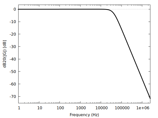

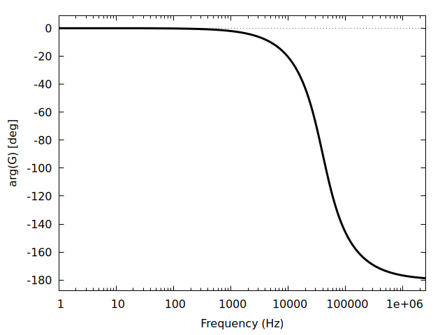
wxplot2d(180/%pi*ArgSymbolic(ev(G_REALIZED(%i*2*%pi*f),%omega_c=2*%pi*40000)),
[f,1,2.5e6],
[logx],
[xlabel,"Frequency (Hz)"],
[ylabel,"arg(G) [deg]"],
[style,[lines,3,11]],
[gnuplot_preamble,"set grid"]);